Implementing Q-learning

Today, we will look at a simple example for implementing Q-learning. Hopefully, you will have a clear understanding after reading this article.

Environment

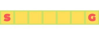
Our environment is a 1x7 grid. S is the Start state and G is the goal state. The agent can only move left or right. The game ends when the agent arrives at G.

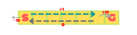
The rewards are as follows: +1 on each step towards G, -10 on illegal step (i.e. moving out of the grid)and finally +10 on reaching G.

Code the agent

def agent(num_iterations=100):
    game = Slider()
    reward_graph = []
    episode_graph = []

    game.reset()
    for episode in range(num_iterations):
        state = 0
        # Used to count the number of moves in a single iteration
        moves = 0
        episodic_reward = 0
        while state != 6:# and moves < 20:
            action = game.get_action(state)
            new_state, reward = game.step(state, action)
            # Temporal Difference
            action = 0 if action == -1 else 1
            temp_diff = reward + max(game.q_table[new_state]) - game.q_table[state][action]
            # Q_learning
            game.q_table[state][action] += game.alpha * temp_diff
            state = new_state
            moves += 1
            episodic_reward += reward
        episode_graph.append(moves)
        reward_graph.append(episodic_reward)

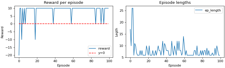
Result

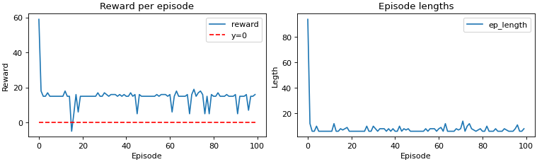
Those sudden spikes are due to exploration vs exploitation tradeoff. Simply put, it explores the environment looking for the best action to take at each time step. This does mean that our agent sometimes selects a bad action. However, this is how our agent learns.

Policy and Q-table

Below is the policy for our trained model.

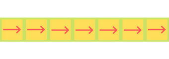
Note: for the Goal state, the policy prefers -> even though the episode restarts when the agent reaches the Goal State. This is down to how the Q-table was initialised and how the policy was chosen.

This is the Q-table after training. Q-table was initialised with zeros rather than randomly. Why don’t you try to implement different things(like random initialization)? This will certainly help in better understanding.

State	<-	->
0	-0.98	1.13
1	0.05	1.25
2	0.12	1.39
3	0.08	1.95
4	0.06	3.55
5	0.18	6.34
6	0.00	0.00

Same agent different Rewards

In this section, we will change the rewards to see how the agent behaves.

First Reward System

Rewards

• +10 for reaching G.
• -10 for an illegal move.

This time, there will be no reward for moving towards the goal state. Let’s see the agent’s performance.

Q-table

The policy remained unchanged, therefore, only the q-table is shown.

S	<-	->
0	-1.31	0.01
1	0.00	0.05
2	0.00	0.25
3	0.01	0.94
4	0.02	2.85
5	0.12	6.34
6	0.00	0.00

Second Reward System

Rewards

• +10 for reaching G
• -10 for an illegal action
• -1 for all other actions.

Q-table

S	<-	->
0	-2.94	-1.82
1	-1.44	-1.44
2	-0.98	-0.98
3	-0.50	-0.06
4	-0.25	2.11
5	-0.04	6.34
6	0.00	0.00

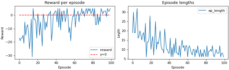
Conclusion

After looking at three different reward systems and their performance, it is worth mentioning that initally the episode length is high. Moreover, the episode length decreases over time. Epsilon-decay is also another concept worth looking into.

The code is available on Github. Tinker with the code and watch your agent learn.